Texas Tree Foundation Analysis Report: Air Quality Analysis

Air Quality Analysis

We have chosen 03/29/2021 air quality data for this analysis. We intend to check if there is any significant statistical difference in air quality and other measurements in different sites such as Medical District Drive, Record Crossing, and Inwood UTSW.

PM 25 Concentration

Based on our visual inspection, the PM 25 concentration of Record Crossing and Inwood UTSW have similar pattern and values but they are different than Medical District Drive values. In order to check if one time series may be used (usefull) to forecast another, we will conduct Granger causality test.

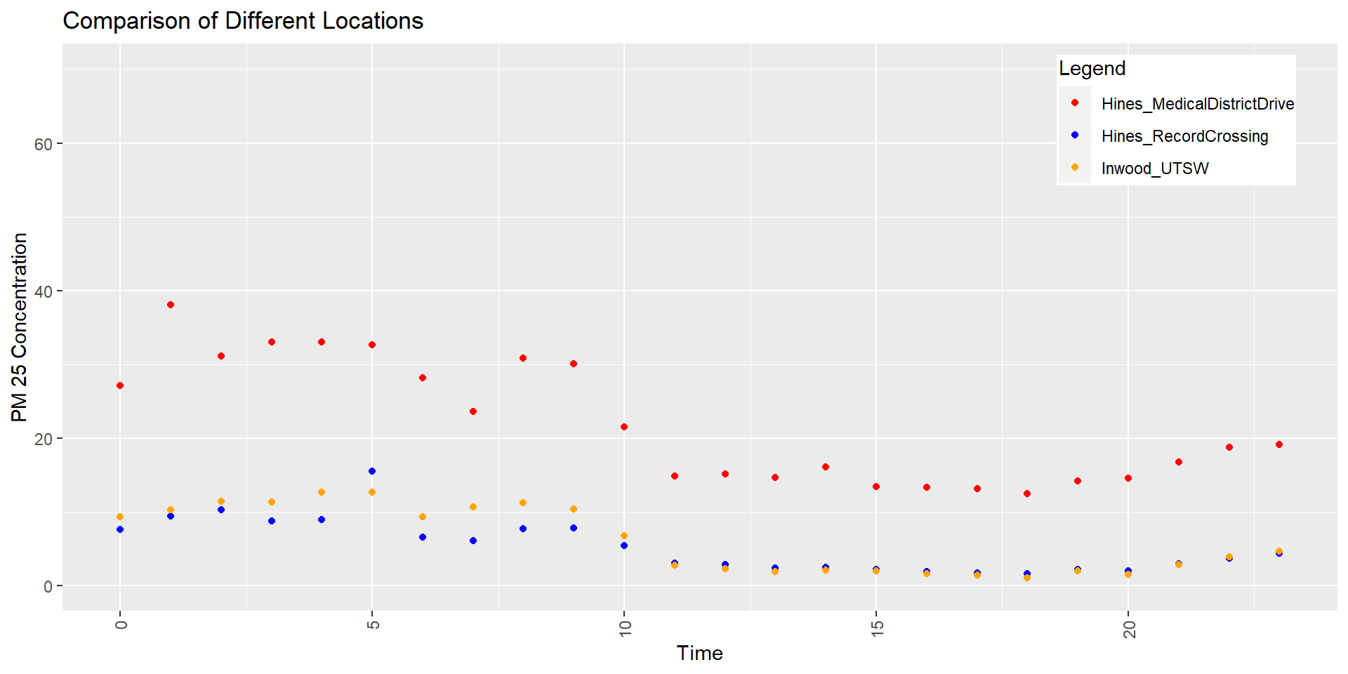
Granger causality test results indicate that Record Crossing time series values are valuable for forecasting the values of Medical District.

Record Crossing vs Inwood

Granger causality test

Model 1: data_iw$pm25_conc ~ Lags(data_iw$pm25_conc, 1:1) + Lags(data_rc$pm25_conc, 1:1)
Model 2: data_iw$pm25_conc ~ Lags(data_iw$pm25_conc, 1:1)
  Res.Df Df      F Pr(>F)
1     20                 
2     21 -1 2.3159 0.1437

Granger causality test

Model 1: data_rc$pm25_conc ~ Lags(data_rc$pm25_conc, 1:1) + Lags(data_md$pm25_conc, 1:1)
Model 2: data_rc$pm25_conc ~ Lags(data_rc$pm25_conc, 1:1)
  Res.Df Df      F    Pr(>F)    
1     20                        
2     21 -1 17.616 0.0004437 ***
---
Signif. codes:  0 '***' 0.001 '**' 0.01 '*' 0.05 '.' 0.1 ' ' 1

Granger causality test

Model 1: data_iw$pm25_conc ~ Lags(data_iw$pm25_conc, 1:1) + Lags(data_md$pm25_conc, 1:1)
Model 2: data_iw$pm25_conc ~ Lags(data_iw$pm25_conc, 1:1)
  Res.Df Df      F Pr(>F)
1     20                 
2     21 -1 1.2614 0.2747

PM 10 Concentration

Based on our visual inspection, the PM 10 concentration of Record Crossing and Inwood UTSW have similar pattern and values but they are different than Medical District Drive values. In order to check if one time series may be used (usefull) to forecast another, we will conduct Granger causality test.

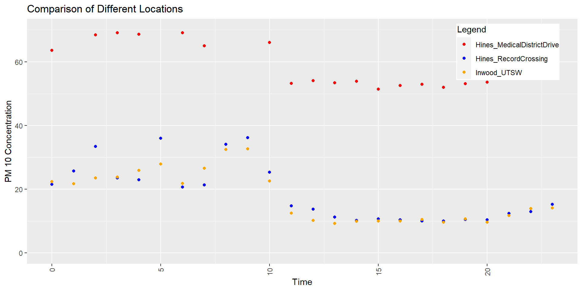
Granger causality test results indicate that Inwood UTSW and Record Crossing time series values are valuable for forecasting the values of Record Crossing and Medical District, respectively.

Record Crossing vs Inwood

Granger causality test

Model 1: data_iw$pm10_conc ~ Lags(data_iw$pm10_conc, 1:1) + Lags(data_rc$pm10_conc, 1:1)
Model 2: data_iw$pm10_conc ~ Lags(data_iw$pm10_conc, 1:1)
  Res.Df Df      F  Pr(>F)  
1     20                    
2     21 -1 6.1424 0.02224 *
---
Signif. codes:  0 '***' 0.001 '**' 0.01 '*' 0.05 '.' 0.1 ' ' 1

Granger causality test

Model 1: data_rc$pm10_conc ~ Lags(data_rc$pm10_conc, 1:1) + Lags(data_md$pm10_conc, 1:1)
Model 2: data_rc$pm10_conc ~ Lags(data_rc$pm10_conc, 1:1)
  Res.Df Df      F  Pr(>F)  
1     20                    
2     21 -1 7.7867 0.01129 *
---
Signif. codes:  0 '***' 0.001 '**' 0.01 '*' 0.05 '.' 0.1 ' ' 1

Granger causality test

Model 1: data_iw$pm10_conc ~ Lags(data_iw$pm10_conc, 1:1) + Lags(data_md$pm10_conc, 1:1)
Model 2: data_iw$pm10_conc ~ Lags(data_iw$pm10_conc, 1:1)
  Res.Df Df      F Pr(>F)
1     20                 
2     21 -1 0.5519 0.4662

NO2 Concentration

Based on our visual inspection, the NO2 concentration of Record Crossing, Inwood UTSW, and Medical District have similar patterns. In order to check if one time series may be used (usefull) to forecast another, we will conduct Granger causality test.

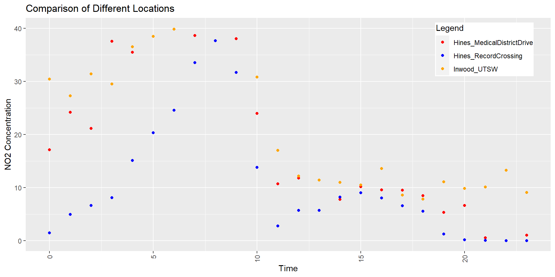
Granger causality test results indicate that Inwood UTSW and Record Crossing time series values are valuable for forecasting the values of Medical District.

Record Crossing vs Inwood

Granger causality test

Model 1: data_iw$no2_conc ~ Lags(data_iw$no2_conc, 1:1) + Lags(data_rc$no2_conc, 1:1)
Model 2: data_iw$no2_conc ~ Lags(data_iw$no2_conc, 1:1)
  Res.Df Df      F Pr(>F)
1     20                 
2     21 -1 0.0783 0.7825

Granger causality test

Model 1: data_rc$no2_conc ~ Lags(data_rc$no2_conc, 1:1) + Lags(data_md$no2_conc, 1:1)
Model 2: data_rc$no2_conc ~ Lags(data_rc$no2_conc, 1:1)
  Res.Df Df     F  Pr(>F)  
1     20                   
2     21 -1 5.596 0.02822 *
---
Signif. codes:  0 '***' 0.001 '**' 0.01 '*' 0.05 '.' 0.1 ' ' 1

Granger causality test

Model 1: data_iw$no2_conc ~ Lags(data_iw$no2_conc, 1:1) + Lags(data_md$no2_conc, 1:1)
Model 2: data_iw$no2_conc ~ Lags(data_iw$no2_conc, 1:1)
  Res.Df Df      F  Pr(>F)  
1     20                    
2     21 -1 7.4091 0.01313 *
---
Signif. codes:  0 '***' 0.001 '**' 0.01 '*' 0.05 '.' 0.1 ' ' 1

Temperature

Based on our visual inspection, the Temperature of Record Crossing, Inwood UTSW, and Medical District have similar patterns. In order to check if one time series may be used (usefull) to forecast another, we will conduct Granger causality test.

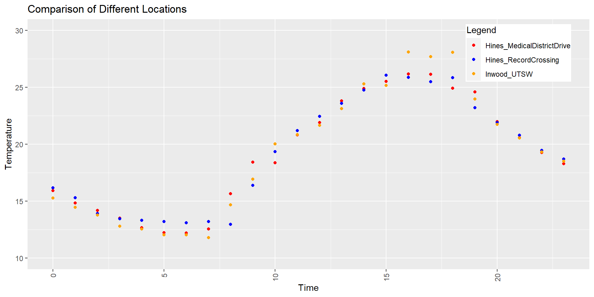
Granger causality test results indicate that Inwood UTSW and Record Crossing time series values are valuable for forecasting the values of Medical District.

Record Crossing vs Inwood

Granger causality test

Model 1: data_iw$temp ~ Lags(data_iw$temp, 1:1) + Lags(data_rc$temp, 1:1)
Model 2: data_iw$temp ~ Lags(data_iw$temp, 1:1)
  Res.Df Df      F Pr(>F)
1     20                 
2     21 -1 0.6708 0.4224

Granger causality test

Model 1: data_rc$temp ~ Lags(data_rc$temp, 1:1) + Lags(data_md$temp, 1:1)
Model 2: data_rc$temp ~ Lags(data_rc$temp, 1:1)
  Res.Df Df      F  Pr(>F)  
1     20                    
2     21 -1 6.8708 0.01636 *
---
Signif. codes:  0 '***' 0.001 '**' 0.01 '*' 0.05 '.' 0.1 ' ' 1

Granger causality test

Model 1: data_iw$temp ~ Lags(data_iw$temp, 1:1) + Lags(data_md$temp, 1:1)
Model 2: data_iw$temp ~ Lags(data_iw$temp, 1:1)
  Res.Df Df      F  Pr(>F)  
1     20                    
2     21 -1 6.4843 0.01922 *
---
Signif. codes:  0 '***' 0.001 '**' 0.01 '*' 0.05 '.' 0.1 ' ' 1

O3 Concentration

Based on our visual inspection, the O3 Concentration of Record Crossing, Inwood UTSW, and Medical District have similar patterns. In order to check if one time series may be used (usefull) to forecast another, we will conduct Granger causality test.

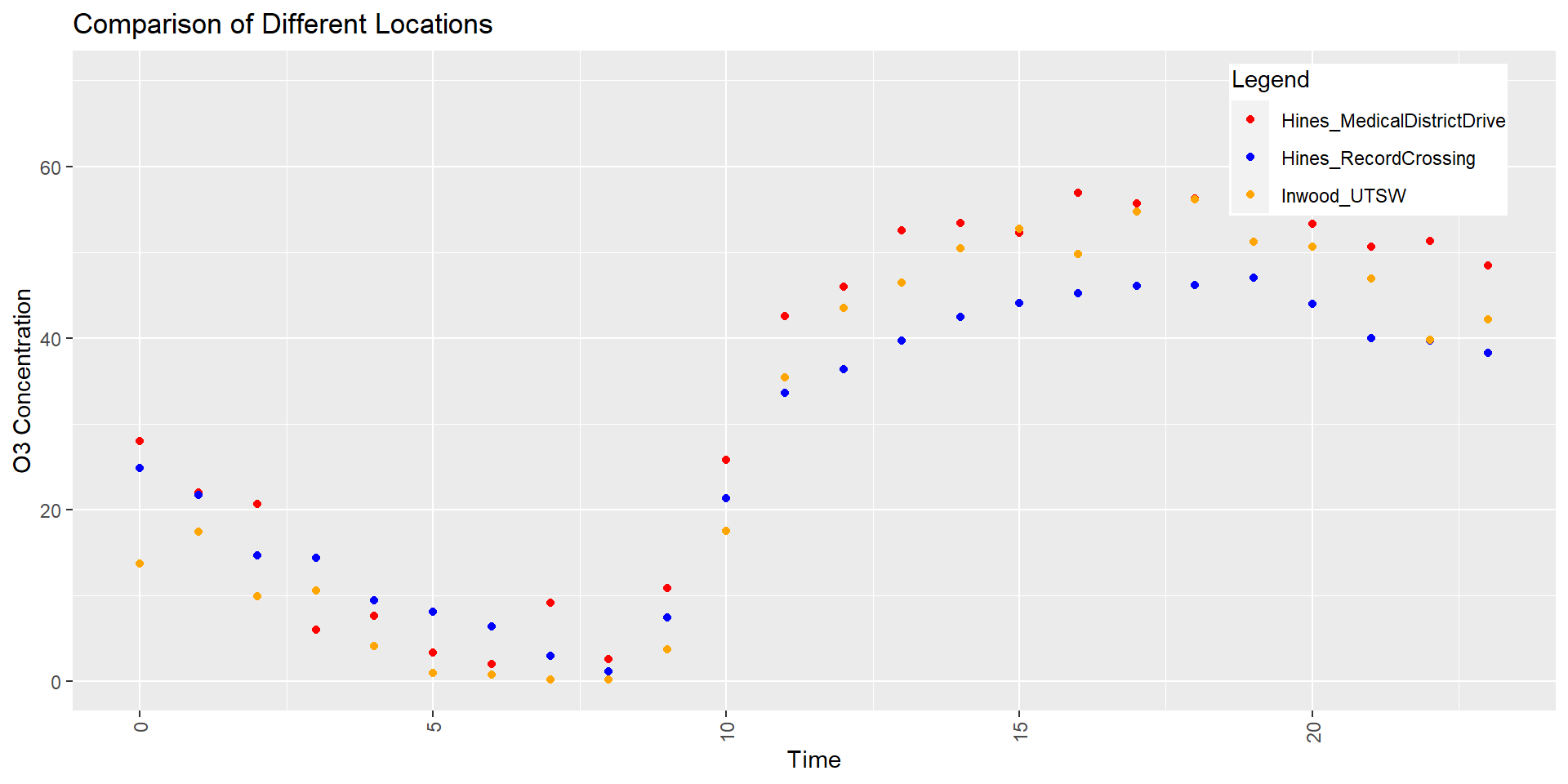
Granger causality test results indicate that Inwood UTSW and Record Crossing time series values are valuable for forecasting the values of Medical District.

Record Crossing vs Inwood

Granger causality test

Model 1: data_iw$o3_conc ~ Lags(data_iw$o3_conc, 1:1) + Lags(data_rc$o3_conc, 1:1)
Model 2: data_iw$o3_conc ~ Lags(data_iw$o3_conc, 1:1)
  Res.Df Df     F Pr(>F)
1     20                
2     21 -1 0.172 0.6827

Granger causality test

Model 1: data_rc$o3_conc ~ Lags(data_rc$o3_conc, 1:1) + Lags(data_md$o3_conc, 1:1)
Model 2: data_rc$o3_conc ~ Lags(data_rc$o3_conc, 1:1)
  Res.Df Df     F  Pr(>F)  
1     20                   
2     21 -1 6.152 0.02214 *
---
Signif. codes:  0 '***' 0.001 '**' 0.01 '*' 0.05 '.' 0.1 ' ' 1

Granger causality test

Model 1: data_iw$o3_conc ~ Lags(data_iw$o3_conc, 1:1) + Lags(data_md$o3_conc, 1:1)
Model 2: data_iw$o3_conc ~ Lags(data_iw$o3_conc, 1:1)
  Res.Df Df      F  Pr(>F)  
1     20                    
2     21 -1 5.8003 0.02579 *
---
Signif. codes:  0 '***' 0.001 '**' 0.01 '*' 0.05 '.' 0.1 ' ' 1